
You can estimate your CdA outdoors using a power meter, reliable speed data and repeated, steady laps. The useful part is making the test consistent enough to distinguish a change in your riding position from a change in wind, slope or measurement error.
This guide explains what to record, how to compare two setups, and where to find the resulting estimates in Peak Watts. The protocol is a practical starting point for your own comparisons. The numerical examples are calculations, not results from a rider who completed this test.
Our bike-weight article held drag area constant to examine the effect of saving mass. Here we investigate that other input: the aerodynamic demand of the rider and bike.
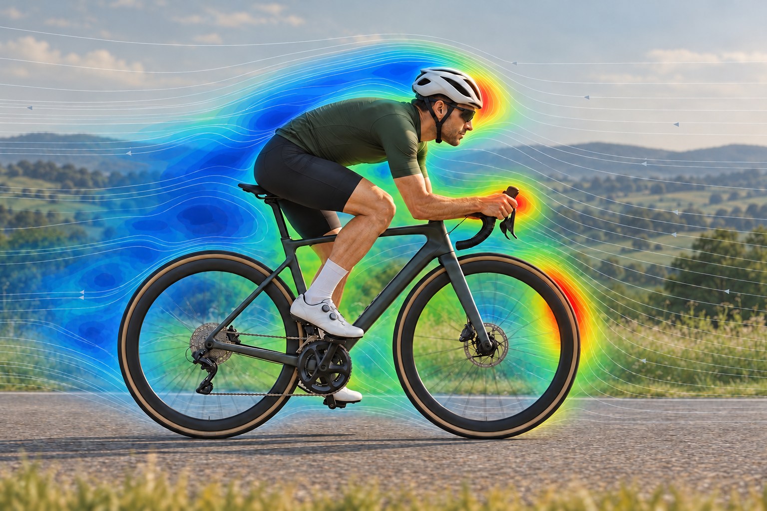
What is CdA?
CdA is drag coefficient multiplied by reference frontal area. Cd describes how an object interacts with the airflow; A is its reference area. Their product, measured in square metres, describes aerodynamic drag for a particular setup and airflow condition.
For cycling, consider the rider and bicycle together. Changing your position changes both the area presented to the air and how air flows around you. Clothing and equipment also affect the result. A smaller frontal silhouette does not necessarily mean proportionally lower drag.
On the road, a power meter supplies one side of an energy balance. Estimate the power used by climbing, rolling resistance, acceleration and drivetrain losses, then attribute the remaining demand to aerodynamics. With speed and environmental data, you can work backwards to an effective CdA. The assumptions behind that calculation matter as much as the displayed decimal places.
What you need to measure CdA on the road
- Measured power. Use a reliable power meter and follow its manufacturer's warm-up and zeroing instructions. Keep the same meter throughout the comparison. Power estimated from speed and a riding model cannot independently establish aerodynamic drag.
- Reliable speed and elevation data. Use a consistent recording source. A correctly configured wheel-speed sensor can help where supported. Elevation matters because even a slight slope changes the power spent against gravity.
- Correct weights and consistent equipment. Check your rider and bike weights. Keep tyres, pressures, clothing, helmet, bottles and carried kit the same when testing a position change.
- A suitable course and weather record. Choose a smooth, nearly level, straight road with room for several uninterrupted minutes. Calm, stable weather makes the comparison easier to interpret.
You can record with Peak Watts or bring in a compatible activity recorded elsewhere. Make sure power, speed and the route are recorded together, and check that weather data is available when reviewing the activity. The phone does not directly measure the airflow around your body.
How to run a controlled CdA field test
1. Choose one change
Call your normal setup A. For B, change one detail, such as hand and forearm position. Pick a position you can hold while looking ahead and controlling the bike normally.
Leave everything else unchanged. Testing a position and a new tyre together makes the result harder to explain: rolling resistance may have changed alongside drag. Decide in advance which interruptions will invalidate a run, such as braking, a passing vehicle or a significant gust.
2. Establish a steady measurement section
Warm up, then reach the intended speed and posture before starting a test lap. Aim for 3–5 minutes of steady riding per measured leg. Hold approximately the same target speed across runs and let measured power reflect the demand. Avoid chasing an exact wattage while also trying to hold an exact speed.
Use a sustainable speed appropriate to the road. Peak Watts can show aerodynamic power at 40 and 50 km/h without you riding that fast. Keep acceleration, braking and turnarounds outside the measured laps, and ride solo, clear of other riders' and vehicles' wakes.
3. Repeat both setups in both directions
Use four blocks in the order A → B → B → A. Each block contains an outward leg and a return leg, with each steady leg marked separately. That gives eight measured legs: two observations per direction for each setup.
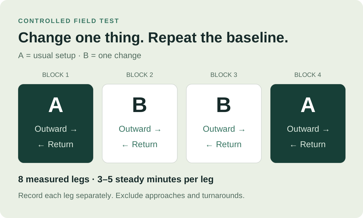
Returning to A helps reveal whether the baseline has drifted during the session. Riding both directions also makes slope or wind differences easier to spot. It does not make wind disappear: opposing wind effects are nonlinear, and conditions can change between legs.
Keep posture, head angle and cadence consistent within each setup. If a run is interrupted, note why and repeat it rather than keeping only the attempts with favorable numbers. Record the setup and direction against each lap number while they are easy to remember.
Find your CdA estimate in Peak Watts
Open the completed activity, go to Laps, select a test leg and find Resistance → CdA Estimate. Detected intervals can also contain estimates, but deliberately marked laps give you clearer boundaries for this test.
The resistance details put wind, gravity and other modeled demands beside the CdA estimate. Check the lap's speed, power, gradient and conditions before comparing its result with another. The activity-analysis page introduces these views.
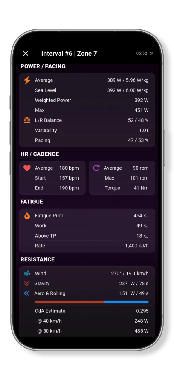
The @ 40 km/h and @ 50 km/h rows translate the estimate into aerodynamic power under common reference conditions: still air and air density of 1.225 kg/m³. This makes the estimates easier to compare. Those watts describe aerodynamic demand alone; total rider power also has to cover the other resistance terms.
Why a lap may have no CdA result
Peak Watts filters out unsuitable samples, including some low-speed, accelerating or strongly wind-assisted riding. A displayed estimate requires more than 60 seconds of accepted CdA data. A lap lasting several minutes may still contain too little usable data.
The current messages include No Weather Data, Short Effort and Inconsistent. Check the available inputs and the steadiness of the effort. The information button explains the need for steady speed, low acceleration and stable wind. A longer lap creates more opportunity to collect useful samples, but does not guarantee an estimate.
Decide whether the difference is repeatable
Record each usable lap's setup, direction, average speed, average power, CdA and any interruptions. Compare A with B within the same direction first, then examine whether the pattern repeats across the blocks. Look at the spread of results as well as their averages.
Suppose two baseline repeats are 0.300 and 0.320 m², while B produces 0.305 m². These hypothetical values do not make a persuasive case for a small improvement: B falls inside the variation already seen in A. More consistent repeats would make a small difference easier to interpret. They would still not remove a shared error in the inputs.
Small slope errors illustrate the problem. At 40 km/h, an 84 kg system on a 0.1% uphill gradient uses about 9.2 W against gravity. At that speed, a 0.01 m² CdA difference corresponds to about 8.4 W of aerodynamic power in still air at the stated density. A small error in the climbing contribution can therefore be similar in size to the change you want to detect.
Weather data may differ from the wind at your position on the road. Rolling resistance is modeled from available bike information or fallback assumptions, and drivetrain losses affect the power available at the wheel. These uncertainties influence the residual attributed to aerodynamics. Keeping the bike, surface and recording equipment consistent helps a position comparison, but does not calibrate every assumption.
Crosswinds add another complication because the apparent airflow has both a speed and an angle. Research on wind yaw and cycling drag explains why a simple inline wind measurement can miss part of that relationship. Favor calm conditions and confirm a promising result in another session before assigning a precise saving to the change.
How much power can a lower CdA save?
In still air, the basic relationships are:
Drag force = ½ × air density × CdA × speed²
Aerodynamic power = ½ × air density × CdA × speed³
Speed is in metres per second, density in kg/m³ and CdA in m². Force is in newtons and power in watts. These resistance relationships form part of the road-cycling power model studied by Martin and colleagues.
At a fixed speed and density, reducing CdA by 10% reduces aerodynamic power by 10%. Because that is only part of the total power requirement, the reduction in total rider power is a smaller percentage when the other demands stay unchanged. Doubling speed multiplies aerodynamic power by eight under the same assumptions.
Consider a hypothetical change from 0.32 to 0.28 m². The following values use still air, density 1.225 kg/m³ and constant speed. They describe the aerodynamic component, before any allowance for drivetrain losses.
| Speed | Aero power at 0.32 m² | Aero power at 0.28 m² | Aero power reduction |
|---|---|---|---|
| 30 km/h | 113.4 W | 99.2 W | 14.2 W |
| 40 km/h | 268.9 W | 235.3 W | 33.6 W |
| 50 km/h | 525.1 W | 459.5 W | 65.6 W |
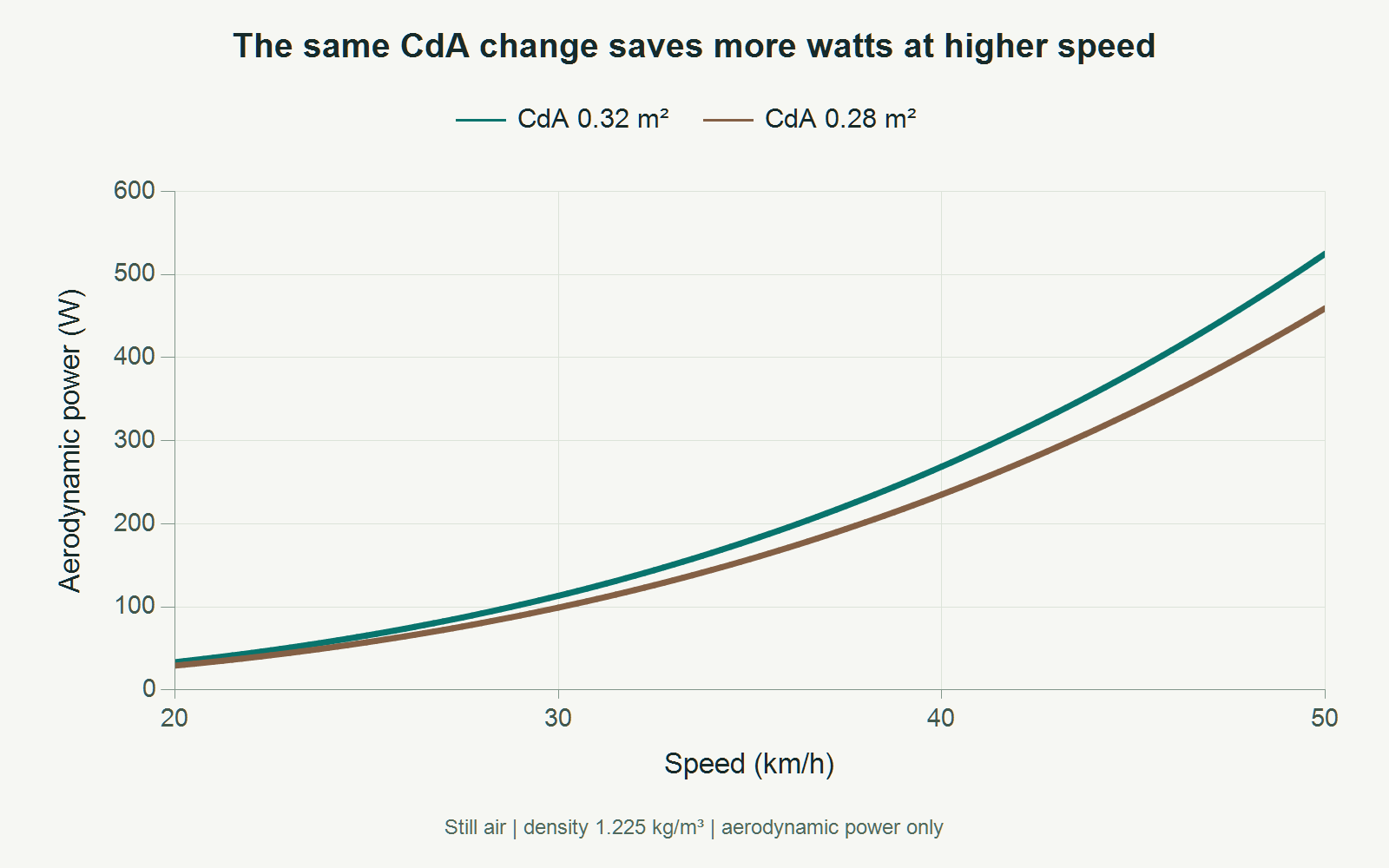
The CdA reduction is 12.5%, so aerodynamic power falls by 12.5% at each speed. The watt saving grows with speed. If you instead hold rider power constant, speed can increase, but the full resistance model is needed to estimate how much. A 12.5% drag-area reduction does not imply a 12.5% shorter finishing time.
In wind, distinguish ground speed from airspeed. Relative airflow determines aerodynamic force, while the mechanical power spent moving along the road also depends on ground speed and force direction. Simply putting airspeed into the cubic still-air formula does not give a general wind calculation.
How does field testing compare with a wind tunnel?
A wind tunnel measures drag force at controlled airflow, then calculates CdA. A field method works backwards from power and motion. An indoor velodrome reduces ambient-wind uncertainty; an outdoor road offers accessibility with less control over conditions.
Martin and colleagues compared field-derived drag areas with wind-tunnel values in six cyclists. Their findings show what carefully controlled field methods can achieve. Their published instructions use a specific protocol with repeated trials and environmental inputs. That study did not validate Peak Watts or establish an accuracy figure for the practical test above.
Use your first session to establish how consistently you can reproduce the baseline. Then investigate one change. An estimate becomes useful when the difference repeats and the position remains comfortable, controllable and compatible with the power you need for the ride.
References and calculation notes
- Martin JC, Milliken DL, Cobb JE, McFadden KL, Coggan AR. Validation of a Mathematical Model for Road Cycling Power. Journal of Applied Biomechanics. 1998;14(3):276–291. doi:10.1123/jab.14.3.276.
- Martin JC, Gardner AS, Barras M, Martin DT. Modeling Sprint Cycling Using Field-Derived Parameters and Forward Integration. Medicine & Science in Sports & Exercise. 2006;38(3):592–597. doi:10.1249/01.mss.0000193560.34022.04. See also the authors' field-test instructions.
- Isvan O. Wind speed, wind yaw and the aerodynamic drag acting on a bicycle and rider. Journal of Science and Cycling. 2015;4(1):42–50.
The power table and chart use ½ × 1.225 × CdA × (km/h ÷ 3.6)³, rounded to 0.1 W. The gradient example uses 84 × 9.81 × sin(arctan(0.001)) × (40 ÷ 3.6). CdA values and repeatability examples are illustrative. App descriptions were checked against the current implementation; the screenshot is an existing feature example.